████████╗██╗  ██╗███████╗███████╗██╗███████╗
╚══██╔══╝██║  ██║██╔════╝██╔════╝██║██╔════╝
   ██║   ███████║█████╗  ███████╗██║███████╗
   ██║   ██╔══██║██╔══╝  ╚════██║██║╚════██║
   ██║   ██║  ██║███████╗███████║██║███████║
   ╚═╝   ╚═╝  ╚═╝╚══════╝╚══════╝╚═╝╚══════╝

Work in progress, just like the thesis itself.

---

Master’s Thesis

#

Programme: Control Engineering & Cybernetics, Integrated Master’s at ITK NTNU Trondheim

Topic: Trajectory reconstruction and sensor fusion for underwater robotics

---

This page is where I will (attempt to) document the work on my master thesis. Right now I’m on the pre-project: building a Kalman filtering and smoothing library from scratch in C++, starting from the simplest possible case and working up toward a strapdown inertial navigation model. Source is on GitHub.

Random walk, Kalman filter, RTS smoother

#

Everything starts with the simplest possible model: a scalar random walk observed through Gaussian noise, $x_{k+1} = x_k + w_k$, $z_k = x_k + v_k$, with $w_k \sim \mathcal{N}(0, Q)$, $v_k \sim \mathcal{N}(0, R)$. Simple enough that the numbers can be checked by hand, which is the point: this is where the core machinery gets built and proven correct before anything harder touches it.

Kalman filter. Predict:

$$ \hat{x}_{k+1|k} = F_k \hat{x}_{k|k}, \qquad P_{k+1|k} = F_k P_{k|k} F_k^\top + Q_k $$

Update:

$$ \begin{aligned} \eta_k &= z_k - H_k \hat{x}_{k|k-1} \\ S_k &= H_k P_{k|k-1} H_k^\top + R_k \\ W_k &= P_{k|k-1} H_k^\top S_k^{-1} \\ \hat{x}_{k|k} &= \hat{x}_{k|k-1} + W_k \eta_k \\ P_{k|k} &= (I - W_k H_k)\, P_{k|k-1}\, (I - W_k H_k)^\top + W_k R_k W_k^\top \end{aligned} $$

The last line is the Joseph form. It’s algebraically identical to the textbook $P_{k|k} = (I - W_kH_k)P_{k|k-1}$, but stays symmetric positive semi-definite even when $W_k$ itself carries numerical error, which the textbook form doesn’t guarantee. Used everywhere in this project instead of the shorter form, for exactly that reason.

RTS smoother. A forward filter pass only ever conditions on past measurements. A smoother makes a second backward pass over the already-filtered estimates, using the whole record, future measurements included, to tighten every estimate in hindsight. For $k = N-1, \dots, 0$:

$$ \begin{aligned} G_k &= P_{k|k}\, F_k^\top\, P_{k+1|k}^{-1} \\ \hat{x}_{k|N} &= \hat{x}_{k|k} + G_k\left(\hat{x}_{k+1|N} - \hat{x}_{k+1|k}\right) \\ P_{k|N} &= P_{k|k} + G_k\left(P_{k+1|N} - P_{k+1|k}\right) G_k^\top \end{aligned} $$

initialized at the filter’s own final estimate, $\hat{x}_{N|N}$, $P_{N|N}$.

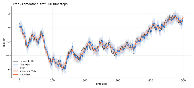
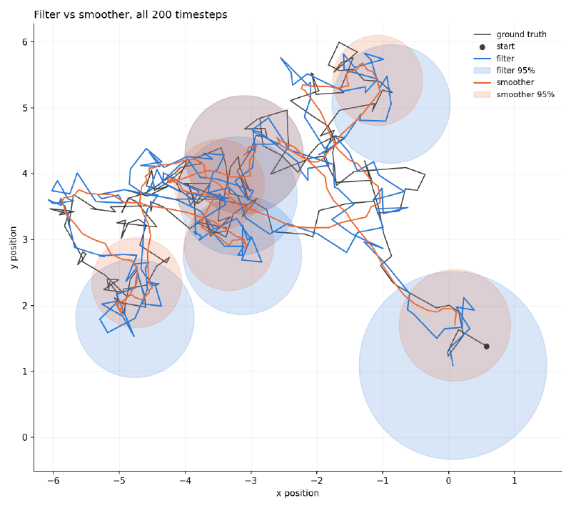
2D repeats the exact same test with vectors instead of scalars, position confidence ellipses instead of bands. The filter and smoother code doesn’t change at all to get there, the dimension lives entirely in the state and measurement vectors, not in the algorithm.

Extended Kalman filter, Extended RTS smoother, and a strapdown INS

#

Both algorithms above generalize directly to a nonlinear model $x_{k+1} = f(x_k) + w_k$, $z_k = h(x_k) + v_k$. The state itself propagates through the real nonlinear $f$ and $h$, only the covariance propagation is linearized, using Jacobians evaluated at the current estimate:

$$ \hat{x}_{k+1|k} = f(\hat{x}_{k|k}), \qquad F_k = \left.\frac{\partial f}{\partial x}\right|_{\hat{x}_{k|k}}, \qquad H_k = \left.\frac{\partial h}{\partial x}\right|_{\hat{x}_{k+1|k}} $$

substituted into the same predict/update equations above, that’s the Extended Kalman Filter. The Extended RTS smoother is the same backward recursion, with $F_k$ now the EKF’s own Jacobian at each step instead of a fixed matrix. Wherever the state has a manifold structure (heading wrapping at $\pm\pi$), addition and subtraction are replaced by explicit composition operators ($\oplus/\ominus$) throughout, both filter and smoother, rather than plain vector $+/-$.

One real wrinkle worth documenting: unlike the filter’s Joseph-form update, the smoother’s covariance recursion has no algebraic PSD guarantee. On the strapdown INS below it does occasionally go indefinite, traced to a combination of $Q$’s structural rank deficiency (more on that below) and a severe scale gap between position variance ($\sim\!10^0$) and bias variance ($\sim\!10^{-10}$) in $P$. Handled for now by masking those timesteps out of the NEES statistic rather than silently miscounting them, not yet fixed at the source.

The model

#

State $x = [p_x,\, p_y,\, \psi,\, u,\, v,\, b_{a_x},\, b_{a_y},\, b_g]^\top \in \mathbb{R}^8$: position, heading, nav-frame velocity, accelerometer bias (both axes), gyro bias. Driven by simulated IMU readings, specific force $a$ and angular rate $\omega$, both corrupted by bias and white noise. Continuous-time kinematics:

$$ \begin{aligned} \dot{p} &= v \\ \dot{\psi} &= \tilde{\omega} \\ \dot{v} &= R(\psi)\,\tilde{a} \\ \dot{b}_a &= -\tfrac{1}{T_a} b_a + w_a, \qquad \dot{b}_g = -\tfrac{1}{T_g} b_g + w_g \end{aligned} $$

where $\tilde{a} = a_{\text{meas}} - b_a$ and $\tilde{\omega} = \omega_{\text{meas}} - b_g$ are the bias-corrected IMU readings, $R(\psi)$ the body-to-nav rotation matrix, and the two biases are Gauss-Markov processes (time constant $T$, driving noise $w$ set so the stationary variance matches a configured value) rather than a plain random walk, so a long run doesn’t let the bias wander off unboundedly.

Discretization. Not plain forward Euler. The rotation is evaluated at the midpoint heading $\psi_{\text{mid}} = \psi_k + \tfrac{1}{2}dt\,\tilde{\omega}$, and position uses constant-acceleration kinematics:

$$ \begin{aligned} \psi_{k+1} &= \psi_k + dt\,\tilde{\omega} \\ a^{\text{nav}} &= R(\psi_{\text{mid}})\,\tilde{a} \\ v_{k+1} &= v_k + dt\, a^{\text{nav}} \\ p_{k+1} &= p_k + dt\, v_k + \tfrac{1}{2} dt^2\, a^{\text{nav}} \\ b_{k+1} &= e^{-dt/T}\, b_k \end{aligned} $$

Using the heading at the middle of the step for the rotation instead of its start is a cheap, standard way to cut heading-linearization error roughly in half per step relative to plain Euler, for one extra rotation-matrix evaluation. The bias update is the exact solution of its Gauss-Markov SDE over one step, nothing to approximate there since it’s already linear.

$F_k$ is the exact Jacobian of this discrete map, so it inherits the midpoint structure: the heading column of the position rows, for instance, carries both a $\tfrac{dt^2}{2}\dot{R}(\psi_{\text{mid}})\tilde{a}$ term and a smaller $\tfrac{dt^3}{4}$ term, the latter from $\psi_{\text{mid}}$’s own dependence on $b_g$ propagating through the chain rule.

$Q_k$ comes from a continuous-time noise input matrix $G$ (how each of the six white noise sources, specific force $\times 2$, angular rate, and the two biases’ driving noise, enters the eight state derivatives) and their intensities $D$:

$$ Q_k \approx dt\, G\, D\, G^\top $$

This is a first-order (Euler-Maruyama) discretization, not the exact Van Loan one, a known simplification left as a TODO in the code. $G$ only touches six of the eight state derivatives directly (position has no row of its own, only indirectly through integrated velocity), so $Q_k$ is structurally rank-deficient, the root cause behind the smoother’s occasional non-PSD covariance mentioned above.

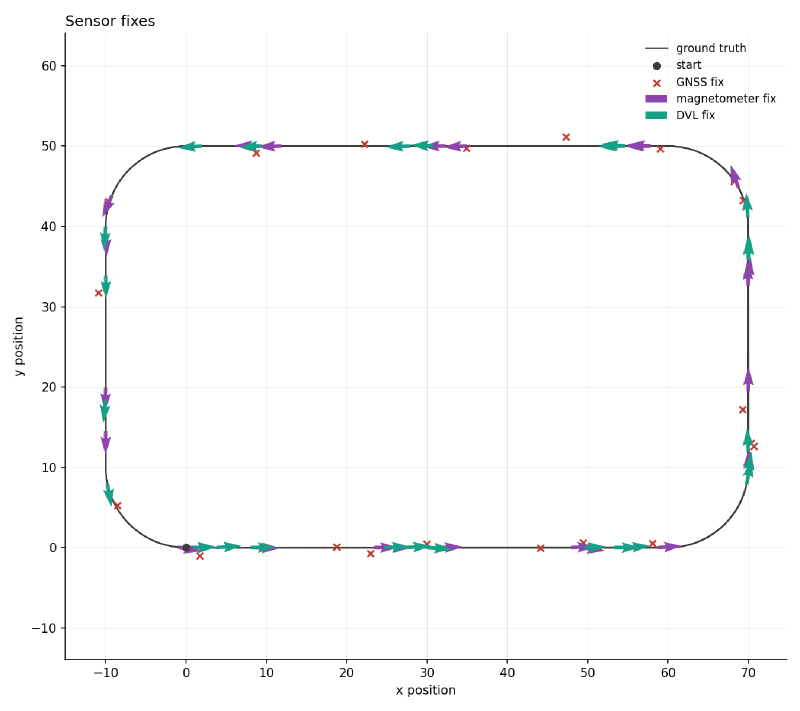
GNSS alone corrects position but says nothing about heading or velocity directly, so two more aiding sensors were added on top: a magnetometer (heading) and a DVL (body-frame velocity from Doppler), each firing on its own independent, irregular schedule and fused into the same filter sequentially within a timestep.

GNSS outages, and why the smoother earns its keep

#

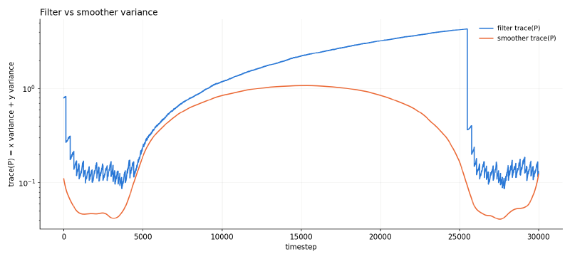
The test I’m most happy with so far: GNSS available for the first and last 15% of a run, denied entirely for the 70% in between, magnetometer and DVL still aiding throughout. The filter’s uncertainty grows steadily through the whole outage and snaps back down the moment GNSS returns. The smoother, since it’s allowed to use both GNSS-aided ends of the run, keeps its peak uncertainty (right in the middle of the outage) below the filter’s uncertainty at almost every other point in the entire run, a direct, visual consequence of the $G_k$ recursion above pulling every estimate toward agreement with both directions of the record.

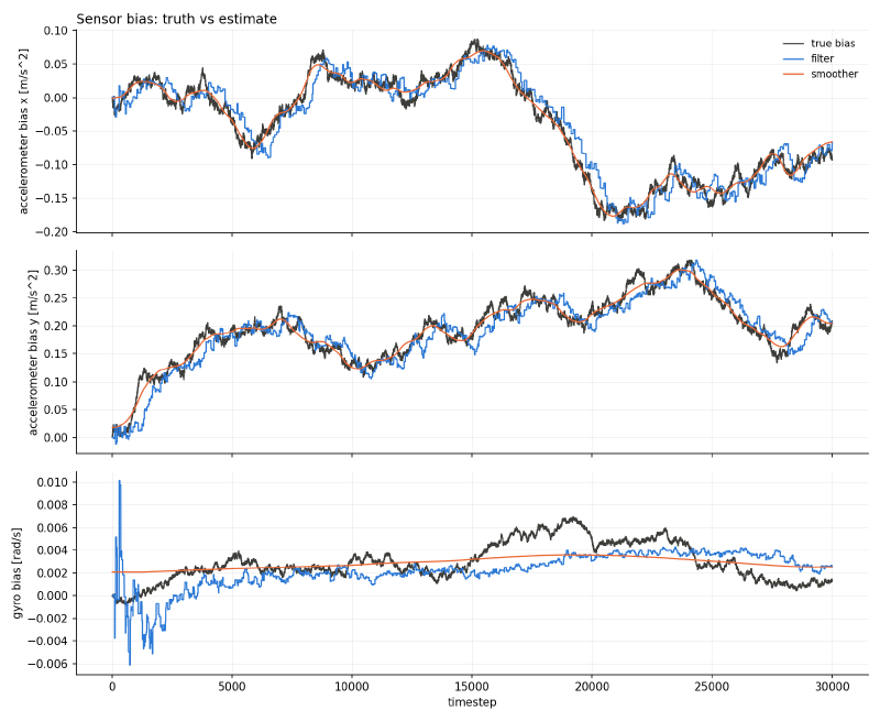
Same run, the IMU bias states themselves: this is exactly where that variance comes from. Accelerometer bias keeps tracking truth closely all the way through the outage, magnetometer and DVL give the filter enough to keep learning it even with GNSS gone. Gyro bias is noisier and drifts further, consistent with it being the hardest of the three to observe in this setup.

What’s next

#

Model mismatch (deliberately wrong filter noise vs. the true noise), an Unscented Kalman Filter for comparison against the Extended one, and eventually a 3D strapdown model with real AUV dynamics (Fossen) once the 2D groundwork is solid. Full writeup and all the numbers live in the repo’s README.

Sources

#

The filtering, smoothing, and consistency-statistics theory throughout this project follows:

Edmund Brekke, Fundamentals of Sensor Fusion, NTNU, 2025.

Simo Särkkä, Bayesian Filtering and Smoothing, Cambridge University Press, 2013.

Marine-craft modeling conventions (body/nav frames, rotation matrices) follow:

Thor I. Fossen, Handbook of Marine Craft Hydrodynamics and Motion Control, 2nd Edition, Wiley, 2021.